LIFT Learning 4D LiDAR Image Fusion Transformer for 3D Object Detection

2023-03-18

Basic Information

Authors: Yihan Zeng, Da Zhang, Chunwei Wang, Zhenwei Miao, Ting Liu, Xin Zhan, Dayang Hao, Chao Ma

Organization: Shanghai Jiao Tong University, Alibaba DAMO Academy

Source: CVPR 2023

Source Code: None

Cite: Zeng, Yihan, et al. “Lift: Learning 4d lidar image fusion transformer for 3d object detection.” Proceedings of the IEEE/CVF Conference on Computer Vision and Pattern Recognition. 2022.

Content

Motivation

We observe that the cross-sensor information may be misaligned over time, as illustrated in Figure 1(a). The reasons lie in two aspects. First, there may exist asynchronous timelines between LiDAR and cameras. Second, the different coordinate systems across sensors introduce spatial misalignment even between synchronized images and point clouds.

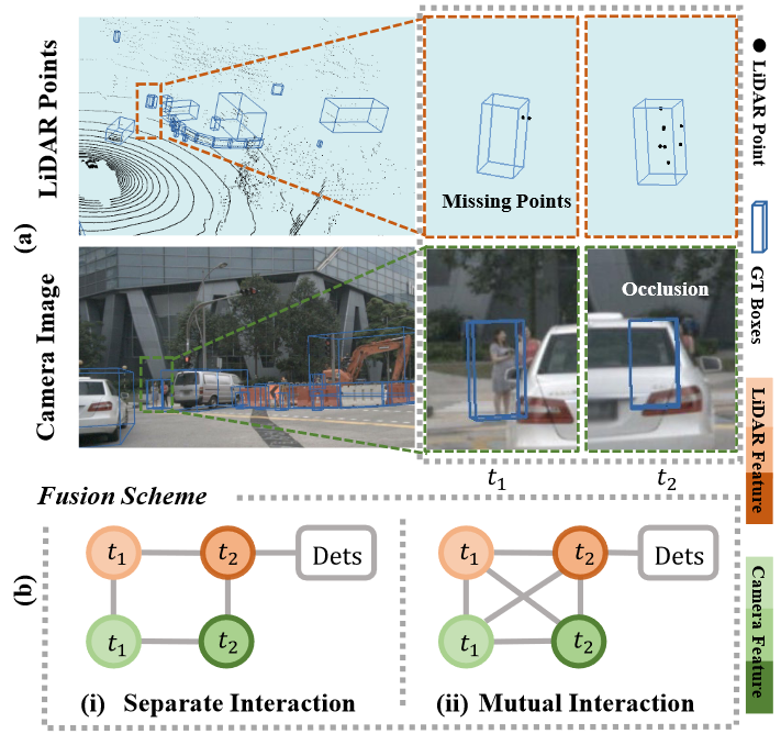
Figure 1. Illustration of the information interaction between sequential cross-sensor data. (a) The misaligned complementary information cross sensors over time. (b) Information fusion scheme: (i) Integrating the cross-sensor data at the corresponding timestamp, then combining the sequential information within sensor streams. (ii) Aggregating information from all timestamps in cross-sensor data streams. Mutual interaction can better connect misaligned complementary information across sensors and time.

Though the very recent work [20] makes an early trial of learning a 4D network, in fact, it uses a preprocessing scheme to concatenate points as temporal fusion, which treats the information interaction as separate parts. By contrast, as shown in Figure 1(b), we propose to explicitly model the mutual correlations between cross-sensor data over time, aiming at the full utilization of misaligned complementary information.

However, it is not feasible to directly apply the standard Transformer architecture for sensor-time fusion in 3D object detection, owing to two facts: 1) The massive amount of 3D points as a sequence input is computationally prohibitive for Transformer. 2) The mutual interaction across sensors and time is beyond the scope of Transformer.

Evaluation

Metric: mAP and report two difficulty levels: LEVEL 1 and LEVEL 2. NDS. Baselines: PointPillars, 3DVID, PointPainting, PointAugmenting.

Datasets

nuScenes, Waymo

Result

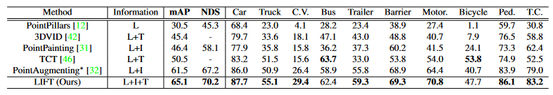
Table 1. Performance comparisons on the nuScenes test set. We report the overall mAP, NDS and mAP for each detection category, where L denotes Lidar modality, I denotes Image modality and T denotes Temporal input. ∗: reproduced results based on PointPillars.

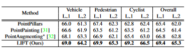
Table 2. Performance comparisons on the Waymo validation set. We report LEVEL 1 and LEVEL 2 mAP(%) for all categories (L 1 and L 2). All models are built on the PointPillars backbone.

Method

n this work, we present LiDAR Image Fusion Transformer (LIFT), an end-to-end single-stage 3D object detection approach, which takes both sequential point clouds and images as input and aims at exploiting their mutual interactions. Figure 2 illustrates the overall architecture of our proposed method, which consists of two main components: (1) Grid Feature Encoder to process the input sequential cross-sensor data into grid features. (2) SensorTime 4D Attention to learn the 4D sensor-time interaction relations given the grid-wise BEV representations.

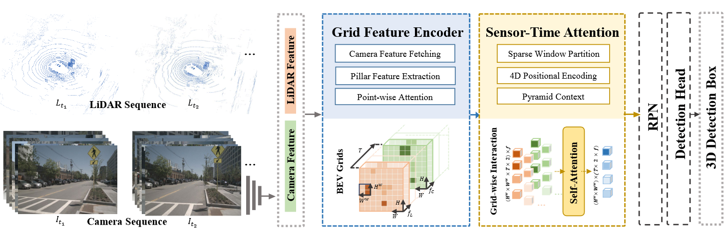
Figure 2. Architecture of LiDAR Image Fusion Transformer (LIFT). LIFT takes both sequential LiDAR point clouds and sequential camera images as input, which are processed into BEV grids by Grid Feature Encoder and fused with Sensor-Time 4D Attention.

Grid Feature Encoder

Compared to a typical point cloud detectors, which learns to classify and localize objects based on single-frame LiDAR point cloud, LIFT takes both sequential point clouds and camera images as input. Specifically, the point clouds can be presented as a sequence of frames $L = \lbrace L_{t_i} \rbrace_{i=1}^T$ where $L_t = \lbrace l_1, \dots, l_{N_L} \rbrace$ consists of $N_L$ LiDAR points $l_i \in R^d$ scattered over the 3D coordinate space. Besides, camera images are presented in time stream $I = \lbrace I_{t_i} \rbrace_{i=1}^T, I_t \in R${U \times V \times 3 \times N_C}$, where U and V denotes the original image size, and $N_C$ is the number of images per scan. For sequential data processing, we use the prior of vehicle pose to remove the effects of ego-motion between different point clouds, then we process each frame following the feature generation pipeline as shown in Figure 3.

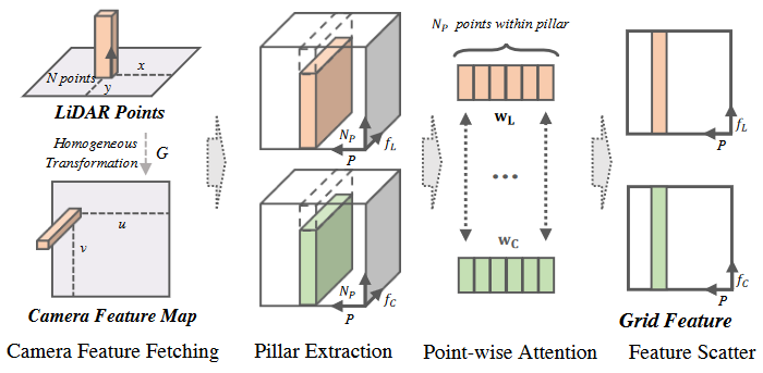
Figure 3. Pipeline of Grid Feature Encoder. We fetch the corresponding camera features for LiDAR points and then capture pillar features for each modality respectively. Besides, point-wise attention is conducted between two modalities within stacked pillars. Finally, the pillar features are scattered into 2D BEV grids.

Camera Feature Fetching

For perspective alignment between modalities, we first align the representations for cross-sensor data input. Specifically, for the camera input, we use the off-the-shelf 2D object detector to extract image features. Then we project point clouds onto the image plane by a prior homogeneous transformation $G \in R^{4 \times 4}$ for fetching the corresponding point-wise image features. There are two benefits. First, the point-level representation aligns images and points in the same 3D coordinate, enabling fine-grained interaction across sensor features. Second, the fetched image feature involves a specific range of receptive field in the image, which helps to alleviate the projection biases between two modalities.

Pillar Feature Extraction.

The number of raw LiDAR points is huge and directly computing point-wise relations is a heavy load to bear. In contrast, the number of BEV grids is small. As such, we encode both point clouds and camera images into the BEV maps separately. Though the projection from 3D points to the 2D space yields information loss of the height dimension, such a loss hardly affects the intrinsic geometry of 3D objects in autonomous-driving scenes.

In more detail, we follow PointPillars to quantize point clouds into P vertical pillars on fixed-size 2D grids. Then we perform linear transformation and max-pooling on each pillar as grid features, which are further scattered into BEV representation $M^L \in R^{H \times W \times f_L}$ , where H and W denote the BEV map size and $f_L$ denotes the feature dimension. Similarly, we obtain the camera features $M^C \in R^{H \times W \times f_C}$ in the BEV as well.

Point-wise Attention.

Inside each pillar, we propose to enhance the pillar encoding via learning a fine-grained correlation among points. Namely, we use two separate learnable linear layers both with $N_p$ outputs to learn weights $w_L$ and $w_C$. Then two weights are applied to the point cloud and the image features over the $N_p$ points within the pillar, respectively. This allows for dynamic information aggregation across two modalities at the fine-grained level with negligible extra cost.

Sensor-Time 4D Attention

To model the mutual correlations of sequential point clouds and camera features, our key motivation is to exploit the self-attention mechanism in Transformer to aggregate complementary information. In this work, the input sequence consists of sequential point cloud and image features. Formally, we assign the grid-wise features from BEV maps $\lbrace M_{t_i}^L, M_{t_i}^C \rbrace_{i=1}^T$ as input tokens. To adapt to 3D object detection, we present three critical designs on top of the classic transformer to model the information interaction across sensors and time, including Sparse Window Partition, Pyramid Context, and 4D Positional Encoding.

Sparse Window Partition

Motivated by the window partition mechanism, we constrain the local self-attention computation within partitioned windows, which largely reduces the number of input tokens. Let the window size $H^w \times W^w$, we obtain $S[\frac{H}{H_w}, \frac{W}{W_w}]$ non-overlapping windows, where S denote the selected sparse non-blank windows. Given the input sequence $F_{in} \in R^{N_F \times f}, $where $N_F = H^w \times W^w \times T \times m $ is the total number of tokens, T denotes the number of frames and m is the number of modalities. we use dot-product attention to model the mutual correlations among input tokens. We formally have:

\[A = Attn(Q(F_{in}), K(F_{in}), V(F_{in}))\]

A nonlinear transformation is applied to the attention weights to produce the output features:

\[F_{out} = MLP(A) + F_{in}\]

Pyramid Context

Another issue with the window-based attention is that the limited local regions may not be sufficient to cover dynamic objects with large motions in adjacent frames. An intuitive solution is to enlarge the size of local windows. However, this would largely increase the parameter volume of attention, yielding heavy computational load.

To enlarge the receptive field with light computation, we consider to resize BEV maps instead, where smaller resolution corresponds to larger receptive regions with fixed window size as demonstrated in Figure 4.

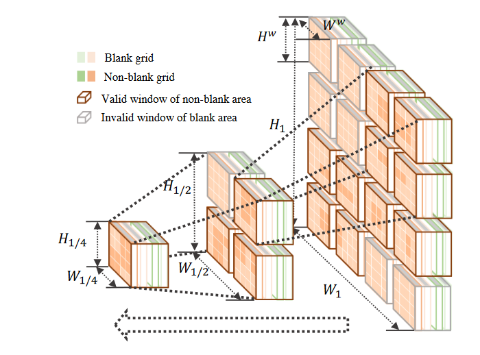
Figure 4. An illustration of pyramid context structure based on sparse windows with $N_M$ = 3. We sparsify the attention window on BEV maps according to whether the partitioned windows include only blank areas. Besides, we adapt the map scale in a pyramid structure, where the down-sampled map provides a larger receptive field.

In particular, we downsample the original BEV map $\lbrace M \rbrace$ with the factor j, and then apply the aforementioned windowbased attention on the packed input $\lbrace \lbrace M \rbrace_j \rbrace^{j \in \lbrace \frac{1}{2^{i-1}} \rbrace_{i=1}^{N_M}}$ with shared parameters, where $N_M$ is the number of scales. Consequently, the attention computation is adapted to:

\[A_j = Attn(Q_j(F_{in}), K_j(F_{in}), V_j(F_{in}))\] \[F_{out} = \sum_j UP(MLP(A_j)) + F_{in}\]

where the upsample operation Up(·) is used to recover the original resolution.

4D Positional Encoding

As vanilla self-attention is unordered, it is crucial to encode the locations of tokens in the input sequence. A common practice of positional encoding is to supplement the feature vector with positional priors. In this work, the candidate tokens in the input sequences are across both sensors and time, which requires 4-Dimensional positional encoding. Thus we introduce a 4D relative position encoder $B \in R^{(H^w)^2 \times (W^w)^2 \times T^2 \times m^2}$ where the positional matrix is parameterized as $\hat B \in R^{(2H^w -1) \times (2W^w-1) \times (2T -1 ) \times (2m -1)}$ and the values in B are taken from $\hat B$.

Hong Huang