Basic Information

Authors: Junbo Yin, Jianbing Shen, Chenye Guan, Dingfu Zhou, Ruigang Yang

Organization: Beijing Lab of Intelligent Information Technology, Baidu Research

Source: CVPR 2020

Source Code: https://github.com/yinjunbo/3DVID (empty)

Cite: Yin, Junbo, et al. “Lidar-based online 3d video object detection with graph-based message passing and spatiotemporal transformer attention.” Proceedings of the IEEE/CVF Conference on Computer Vision and Pattern Recognition. 2020.

Content

Motivation

The majority of current 3D object detection approaches follow the single-frame detection paradigm, while few of them perform detection in the point cloud video. A point cloud video is defined as a temporal sequence of point cloud frames.

Detection in single frame may suffer from several limitations due to the sparse nature of point cloud. In particular, occlusions, longdistance and non-uniform sampling inevitably occur on a certain frame, where a single-frame object detector is incapable of handling these situations, leading to a deteriorated performance, as shown in Fig 1.

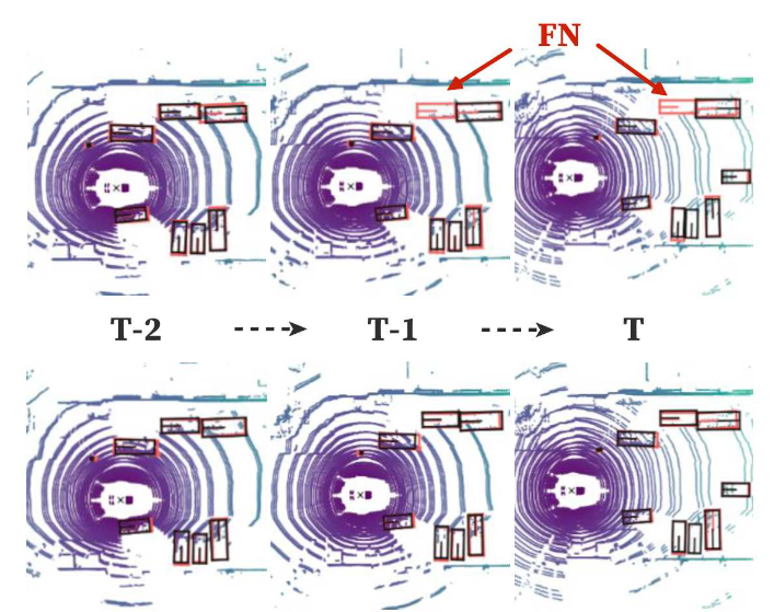
Figure 1. Occlusion situation in autonomous driving scenarios. Typical single-frame 3D object detector, often leads to false-negative (FN) results (top row). In contrast, our online 3D video object detector can handle this (bottom row). The grey and red boxes denote the predictions and ground-truths, respectively.

However, a point cloud video contains rich spatiotemporal information of the foreground objects, which can be explored to improve the detection performance. The major concern of constructing a 3D video object detector is how to model the spatial and temporal feature representation for the consecutive point cloud frames. In this work, we propose to integrate a graph-based spatial feature encoding component with an attention-aware spatiotemporal feature aggregation component, to capture the video coherence in consecutive point cloud frames, which yields an end-to-end online solution for the LiDAR-based 3D video object detection.

A potential problem with current 3D object detectors lies in that they only focus on a locally aggregated feature. To further enlarge the receptive fields, they have to apply the stride or pooling operations repeatedly, which will cause the loss of the spatial information. To alleviate this issue, we propose a novel graph-based network, named Pillar Message Passing Network (PMPNet), which treats a non-empty pillar as a graph node and adaptively enlarges the receptive field for a node by aggregating messages from its neighbors.

After obtaining the spatial features of each input frame, we assemble these features in our spatiotemporal feature aggregation component. Since ConvGRU has shown promising performance in the 2D video understanding field, we suggest an Attentive Spatiotemporal Transformer GRU (AST-GRU) to extend ConvGRU to the 3D field through capturing dependencies of consecutive point cloud frames with an attentive memory gating mechanism.

Evaluation

Metric: mAP@IOU0.5

Implementation Details: For each keyframe, we consider the point clouds within range of [−50, 50] × [−50, 50] × [−5, 3] meters along the X, Y and Z axes.

Baselines : VIPL_ICT, MAIR, PointPillars, SARPNET, WYSIWYG, Tolist

Datasets

nuScenes

Result

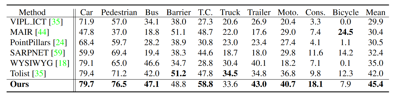
Table 1. Quantitative detection results on the nuScenes 3D object detection benchmark. T.C. presents the traffic cone. Moto. and Cons. are short for the motorcycle and construction vehicle, respectively. Our 3D video object detector outperforms the single-frame detectors, achieving state-of-the-art performance on the leaderboard.

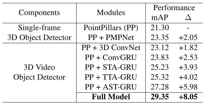
Table 2. Ablation study for our 3D video object detector. PointPillars is the reference baseline for computing the relative improvement ($\Delta$).

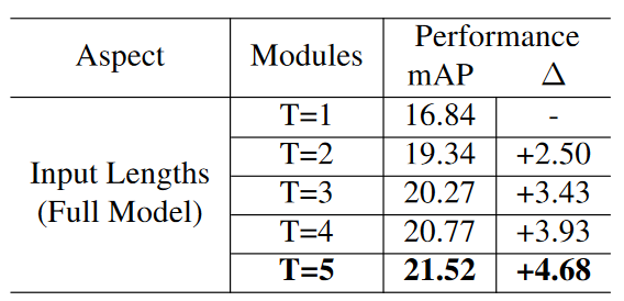
Table 3. Ablation study for the input lengths. Detection results with one input frame are used as the reference baseline.

Method

Overview

As shown in Fig. 2, it consists of a spatial feature encoding component and a spatiotemporal feature aggregation component. Given the input sequences $\lbrace I_t \rbrace_{t=1}^T$ with $T$ frames, we first convert the point cloud coordinates from the previous frames $\lbrace I_t \rbrace_{t=1}^{T-1}$ to the current frame $I_T$ using the GPS data, so as to eliminate the influence of the ego-motion and align the static objects across frames. Then, in the spatial feature encoding component, we extract features for each frame with the Pillar Message Passing Network (PMPNet) and a 2D backbone, producing sequential features $\lbrace X_t \rbrace_{t=1}^T$. After that, these features are fed into the Attentive Spatiotemporal Transformer Gated Recurrent Unit (AST-GRU) in the spatiotemporal feature aggregation component, to generate the new memory features $\lbrace H_t \rbrace_{t=1}^T$. Finally, a RPN head is applied on $\lbrace H_t \rbrace_{t=1}^T$ to give the final detection results $\lbrace Y_t \rbrace_{t=1}^T$.

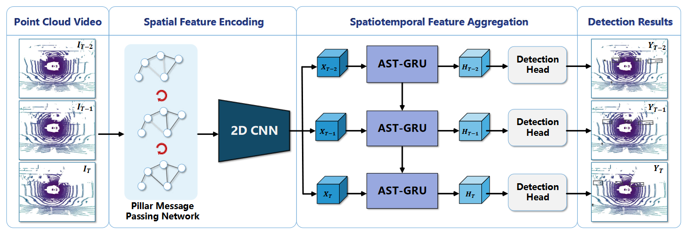
Figure 2. Our online 3D video object detection framework includes a spatial feature encoding component and a spatiotemporal feature aggregation component. In the former component, a novel PMPNet is proposed to extract the spatial features of each point cloud frame. Then, features from consecutive frames are sent to the AST-GRU in the latter component, to aggregate the spatiotemporal information with an attentive memory gating mechanism.

Pillar Message Passing Network(PMPNet)

Previous point cloud encoding layers (e.g., the VFE layers and the PFN) for voxel-based 3D object detection typically encode each voxel or pillar separately, which limits the expressive power of the grid-level representation due to the small receptive field of each local grid region. Our PMPNet instead seeks to explore the rich spatial relations among different gird regions by treating the non-empty pillar grids as graph nodes. Such design effectively reserves the non-Euclidean geometric characteristics of the original point clouds and enhance the output pillar features with a non-locality property.

Given an input point cloud frame $I_t$, we first uniformly discretize it into a set of pillars $P$. Then, PMPNet maps the resultant pillars to a directed graph $G = (V, E)$, where node $v_i \in V$ represents a non-empty pillar $P_i \in P$ and edge $e_{i,j} \in E$ indicates the message passed from node $v_i$ to $v_j$. For reducing the computational overhead, we define $G$ as a k-nearest neighbor (k-NN) graph, which is built from the geometric space by comparing the centroid distance among different pillars.

To explicitly mine the rich relations among different pillar nodes, PMPNet performs iterative message passing on $G$ and updates the nodes state at each iteration step. Concretely, given a node $v_i$, we first utilize a pillar feature network (PFN) to describe its initial state $h_i^0 = F_{PFN}(P_i) \in R^L$ at iteration step $s = 0$ where $h_i^0$ is a $L$-dim vector and $P_i$ presents a pillar containing $N$ LiDAR points, with each point parameterized by D dimension representation.

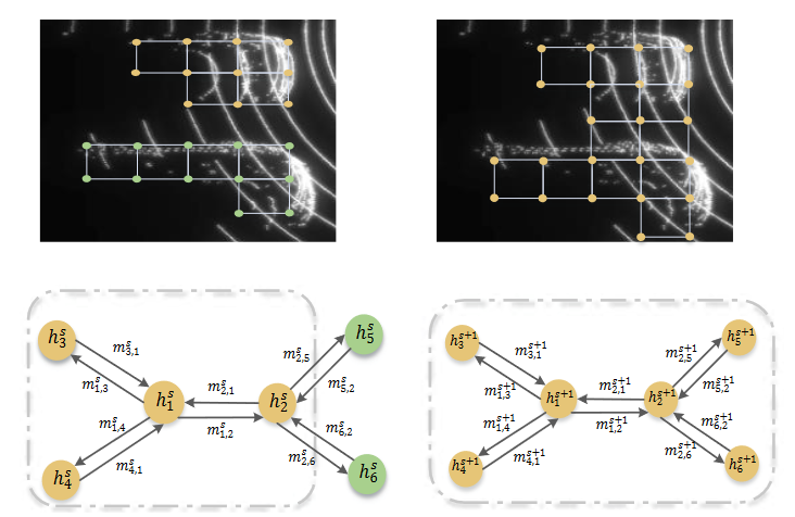
Figure 3. Illustration of one iteration step for message propagation, where $h_i$ is the state of node $v_i$ . In step $s$, the neighbors for $h_1$ are $\lbrace h_2, h_3, h_4 \rbrace$ (within the gray dash line), presenting the pillars in the top car. After aggregating messages from the neighbors, the receptive field of $h_1$ is enlarged in step $s + 1$, indicating the relations with nodes from the bottom car are modeled.

Next, we elaborate on the message passing process. One iteration step of message propagation is illustrated in Fig. 3. At step s, a node $v_i$ aggregates information from all the neighbor nodes in the k-NN graph. We define the incoming edge feature from node $v_j$ as $e_{j,i}^s$, indicating the relation between node $v_i$ and $v_j$. Inspired by [1], The incoming edge feature $e_{j,i}^s$ is given by

which is an asymmetric function encoding the local neighbor information. Accordingly, we have the message passed from $v_j$ to $v_i$ , which is denoted as:

where $f$ is parameterized by a fully connected layer.

After computing all the pair-wise relations between $v_i$ and the neighbors $v_j \in N_{v_i}$, we summarize the received k messages with a maximum operation:

Then, we update the node state $h_i^s$ with $h_i^{s+1}$ for node $v_i$. The update process should consider both the newly collected message $m_i^{s+1}$ and the previous state $h_i^s$. The update process is then formulated as follows:

Consequently, after the totally $S$ iteration steps, node $v_i$ is able to aggregate information from the high-order neighbors.

Therefore, after performing the iterative message passing, the encoded pillar features are then scattered back as a 3D tensor $\hat I_t \in R^{W \times H \times C}$, which can be further exploited by the 2D CNNs. Here, we leverage the backbone network to further extract features for $\hat I_t$:

where $F_B$ denotes the backbone network and $X_t$ is the spatial features of $I_t$ .

Attentive Spatiotemporal Transformer GRU

Since the sequential features $\lbrace X_t \rbrace^T_{t=1}$ produced by the spatial feature encoding component are regular tensors, we can employ the ConvGRU to fuse these features in our spatiotemporal feature aggregation component.** However, it may suffer from two limitations when directly applying the ConvGRU.** On the one hand, the interest objects are relatively small in the bird’s eye view compared with those in the 2D images. This may cause the background noise to dominate the results when computing the memory. On the other hand, though the static objects can be well aligned across frames using the GPS data, the dynamic objects with large motion still lead to an inaccurate new memory.

To address the above issues, we propose the AST-GRU to equip the vanilla ConvGRU[2] with a spatial transformer attention (STA) module and a temporal transformer attention (TTA) module. As illustrated in Fig. 4, the STA module stresses the foreground objects in $\lbrace X_t \rbrace^T_{t=1}$ and produces the attentive new input $\lbrace X_t’ \rbrace^T_{t=1}$, while the TTA module aligns the dynamic objects in $\lbrace H_{t-1} \rbrace^T_{t=1}$ amd $\lbrace X_t’ \rbrace^T_{t=1}$ and outputs the attentive old memory $\lbrace H_{t-1}’ \rbrace^T_{t=1}$. Then,$\lbrace X_t’ \rbrace^T_{t=1}$ and $\lbrace H_{t-1}’ \rbrace^T_{t=1}$ , and further produce the final detections $\lbrace Y_t \rbrace^T_{t=1}$.

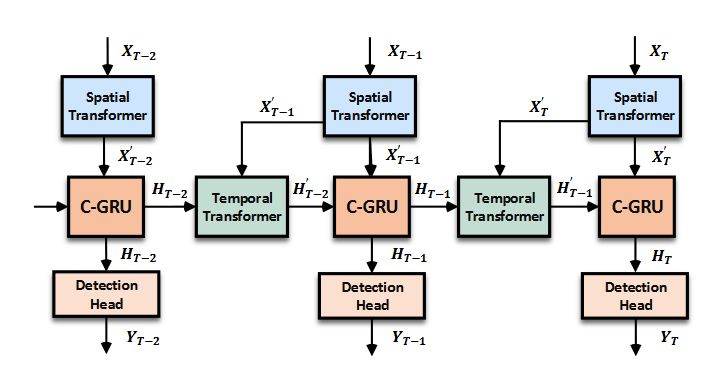
Figure 4. The detailed architecture of the proposed ASTGRU, which consists of a spatial transformer attention (STA) module and a temporal transformer attention (TTA) module. ASTGRU models the dependencies of consecutive frames and produces the attentive new memory $\lbrace H_t \rbrace^T_{t=1}$

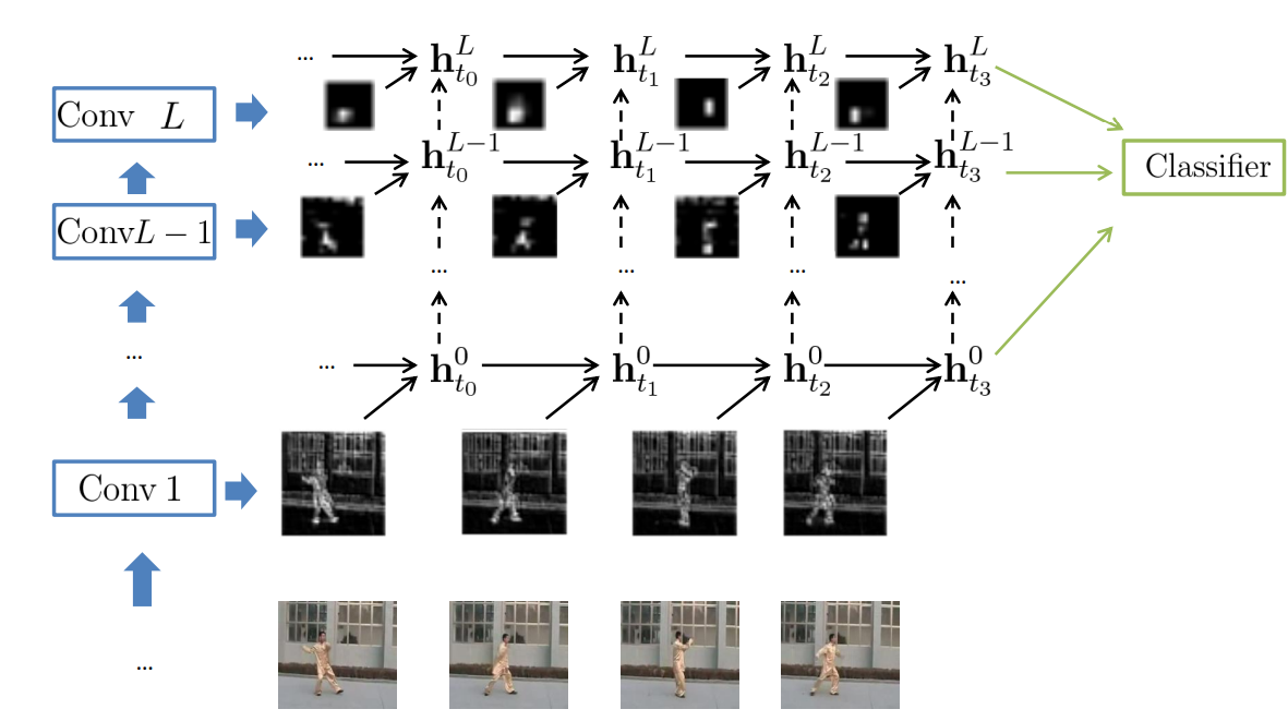
Figure 5. High-level visualization of ConvGRU

Spatial Transformer Attention.

The core idea of the STA module is to attend each pixel-level feature $x \in X_t$ with a rich spatial context, to better distinguish a foreground object from the background noise. (In fact, it is just a self-attention module.)

Temporal Transformer Attention.

Given $H_{t-1}$ and $X_t’$, we want to obtain the attentive memory $H_{t-1}’$. The core is to attend the queries in $H_{t-1}$ with adaptive supporting key regions computed by integrating the motion information.

First we compute deformation offset

where the channel number $2r^2$ denotes the offsets in the x-y plane for the $r \time r$ convolutional kernel.

Then we get the attentive output $h’_q$ of query $h_q$ is given by:

$f_V(h_k)$ is an identity function and $w_m$ acts as the weights in different attention heads, with each head corresponding to a sampled key position$k \in N_q$. $G(\cdot, \cdot)$ is the attention weight defined by a bilinear interpolation function

The intuition is that, in the motion map, the features response of the static objects is very low since they have been spatially aligned in $H_{t-1}$ and $X_t’$, while the features response of the dynamic objects remains high. Therefore, we integrate $H_{t-1}$ with the motion map, to further capture the motions of dynamic objects.

Comments

Pros

1. Motion fusion is impressive.

Cons

1. Table 3 shows full model perform bad when T=1. When T=5, full model is still worse than single-frame model in Table 2.
2. Why the author choose KNN instead of self attention?

Further work

Extending the theoretical framework to adaptive optimization methods or gossip-based training method.

Comments

(need further experiment)

References

[1] Yue Wang, Yongbin Sun, Ziwei Liu, Sanjay E Sarma, Michael M Bronstein, and Justin M Solomon. Dynamic graph cnn for learning on point clouds. ACM Transactions on Graphics, 38(5):146, 2019. 4 [2] Nicolas Ballas, Li Yao, Chris Pal, and Aaron Courville. Delving deeper into convolutional networks for learning video representations. In ICLR, 2016. 2, 4, 5 [3] Wenjie Luo, Bin Yang, and Raquel Urtasun. Fast and furious: Real time end-to-end 3d detection, tracking and motion forecasting with a single convolutional net. In CVPR, 2018. 3, 5, 8